DNN Hog Price Prediction - Dear-夜下小灼

Outlines
Why Now Neural Networks
Data Exploring
Feature Engineering
Feature Scaling
Model Designing
Model Training
Model Predicting
Data Visualization
Dataset & Full Code

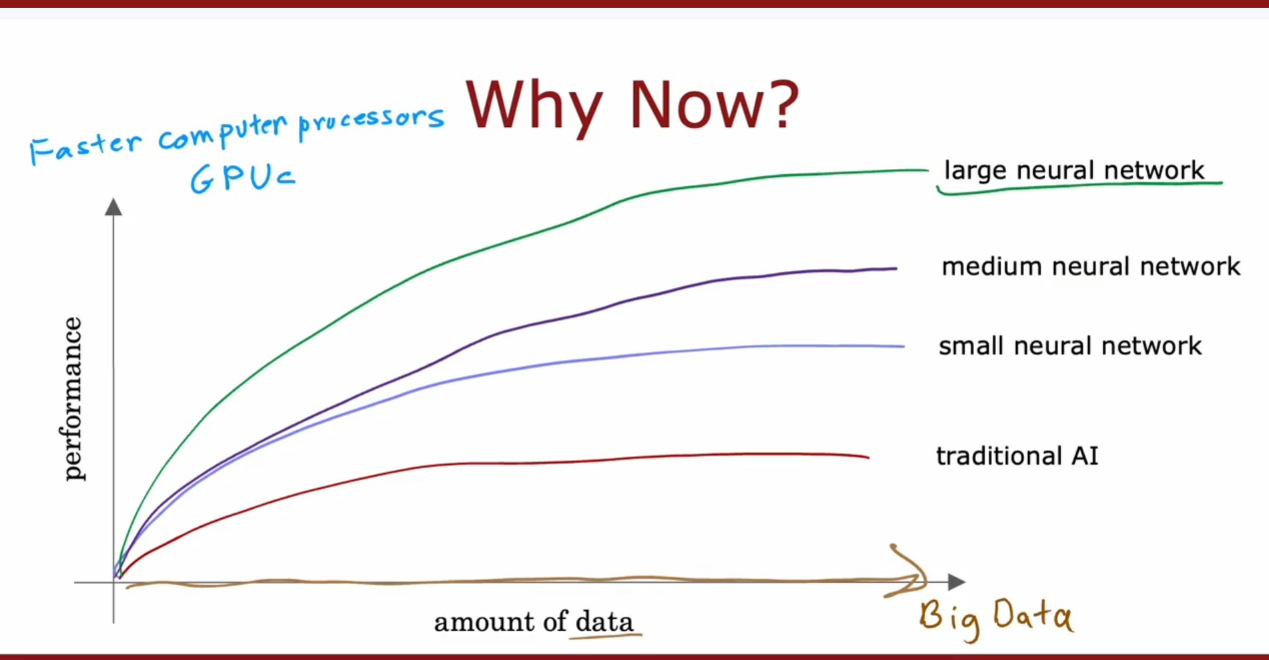
Why Now Neural Networks

“The idea of neural networks have been around for many decades, so a few people have asked me hey Andrew，why now why is it that only in the last handful of years that neural networks have really taken off, this is a picture I draw for them”——Andrew Ng

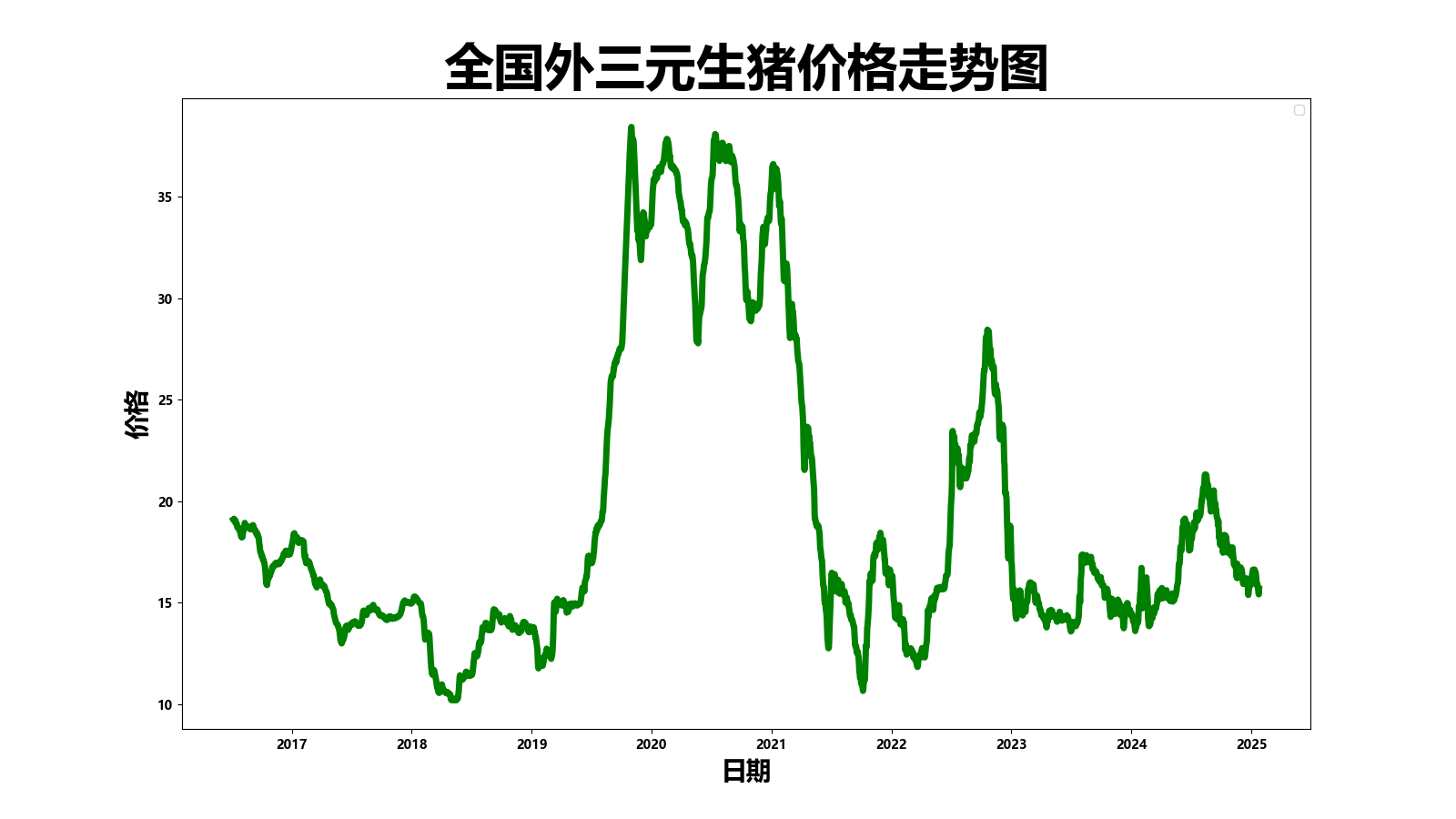
Data Exploring

7/7/2016 19.1
8/7/2016 19.07
9/7/2016 19.13
10/7/2016 19.09
......
22/1/2025 15.54
23/1/2025 15.42
24/1/2025 15.69

Python

import pandas as pd
import matplotlib
import matplotlib.pyplot as plt


matplotlib.use('TkAgg')
matplotlib.rc("font", family='MicroSoft YaHei', weight="bold")


def exploration():
    realDF = pd.read_table("../dataset/data", header=None, names=['dmy', 'price'], sep=" ")
    realDF['dmy'] = pd.to_datetime(realDF['dmy'], format="%d/%m/%Y")
    realDF.sort_values(by='dmy', inplace=True)

    plt.figure(figsize=(16, 9), dpi=100)
    plt.title("全国外三元生猪价格走势图", fontsize=40, weight="bold")
    plt.xlabel("日期", fontsize=20, weight="bold")
    plt.ylabel("价格", fontsize=20, weight="bold")
    plt.plot(realDF['dmy'], realDF['price'], '-g', linewidth=5.0)
    plt.legend()
    plt.show()


if __name__ == '__main__':
    exploration()

Feature Engineering
Here we expand the default format “%d/%m/%Y” to day, month, and year

Python

def dataExpand(df):
    print("dataExpand is called...")
    _df = pd.concat([df, df['dmy'].str.split('/', expand=True)], axis=1)
    df['d'], df['m'], df['y'] = _df[0].astype(float), _df[1].astype(float), _df[2].astype(float)
    pass

Feature Scaling
This step is important to limit the scope of feature value to a proper range and boost the training

\(
{\huge x = \frac{x – \mu }{\sigma} }
\)

Python

def _featureScale(nDArray, mu=None, sigma=None):
    print("_featureScale is called...")
    if mu is None or sigma is None:
        mu = nDArray[:, :-2].mean(axis=0)
        sigma = nDArray[:, :-2].astype(np.float32).std(axis=0)
    nDArray[:, :-2] = (nDArray[:, :-2] - mu) / sigma
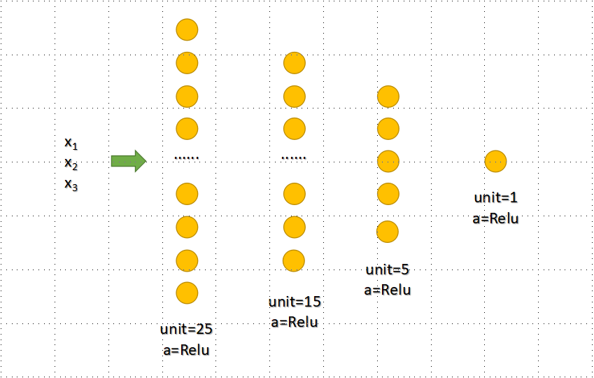
    return mu, sigma

Model Designing

Model Training

Python

def training(self, learningRate=1e-3, epochs=200):
    print("training is called...")
    self.model = Sequential([
        Dense(units=25, activation='relu'),
        Dense(units=15, activation='relu'),
        Dense(units=5, activation='relu'),
        Dense(units=1, activation='relu'),
    ])
    self.model.compile(optimizer=Adam(learning_rate=learningRate), loss=MeanSquaredError())
    history = self.model.fit(self.trainX, self.trainY, epochs=epochs)
    return history.history['loss'][-1]
    pass

Epoch 1/200
78/78 [==============================] - 0s 635us/step - loss: 412.6936
Epoch 2/200
78/78 [==============================] - 0s 557us/step - loss: 286.1414
Epoch 3/200
78/78 [==============================] - 0s 590us/step - loss: 96.9163
Epoch 4/200
78/78 [==============================] - 0s 583us/step - loss: 69.8008
Epoch 5/200
78/78 [==============================] - 0s 622us/step - loss: 65.8830
Epoch 6/200
78/78 [==============================] - 0s 621us/step - loss: 62.9686
Epoch 7/200
78/78 [==============================] - 0s 596us/step - loss: 59.6960
Epoch 8/200
78/78 [==============================] - 0s 570us/step - loss: 55.9135
Epoch 9/200
78/78 [==============================] - 0s 570us/step - loss: 51.6902
Epoch 10/200
78/78 [==============================] - 0s 570us/step - loss: 47.3465
......
Epoch 191/200
78/78 [==============================] - 0s 583us/step - loss: 1.3342
Epoch 192/200
78/78 [==============================] - 0s 583us/step - loss: 1.3265
Epoch 193/200
78/78 [==============================] - 0s 557us/step - loss: 1.3573
Epoch 194/200
78/78 [==============================] - 0s 570us/step - loss: 1.3004
Epoch 195/200
78/78 [==============================] - 0s 583us/step - loss: 1.2744
Epoch 196/200
78/78 [==============================] - 0s 584us/step - loss: 1.2893
Epoch 197/200
78/78 [==============================] - 0s 570us/step - loss: 1.3706
Epoch 198/200
78/78 [==============================] - 0s 583us/step - loss: 1.2538
Epoch 199/200
78/78 [==============================] - 0s 597us/step - loss: 1.2335
Epoch 200/200
78/78 [==============================] - 0s 570us/step - loss: 1.2402

Model Predicting

Python

def prediction(self, testX, testY, testID):
    pre = self.model.predict(testX)
    pre = pre.flatten()
    t = pd.DataFrame({'date': testID, 'predictY': pre, 'realY': testY})
    t['predictY'] = t['predictY'].apply(lambda x: format(x, '0.2f'))
    print(t.head(20))
    t[['date', 'predictY']].to_csv("./dataset/predict", header=None, sep=" ", index=None)
    print("prediction saved")
    pass

          date predictY  realY
0     2/4/2017    15.10  15.94
1   26/10/2016    16.99  16.38
2    6/12/2019    34.25  34.04
3    30/9/2019    29.37   27.5
4    23/1/2020    37.14  36.33
5    22/4/2020    32.93  33.24
6    29/8/2020    36.25  36.81
7   29/12/2016    16.42  17.58
8    31/5/2022    16.41  15.68
9    16/4/2022    13.32  12.87
10   10/9/2020    35.47   36.5
11   28/3/2021    25.53  26.29
12  24/11/2022    22.28  24.36
13    6/5/2022    14.82   15.0
14   26/5/2019    15.87  14.96
15    8/3/2023    14.55   15.8
16    4/9/2021    14.50  14.08
17   26/5/2022    15.87  15.75
18    5/9/2023    17.37  16.66
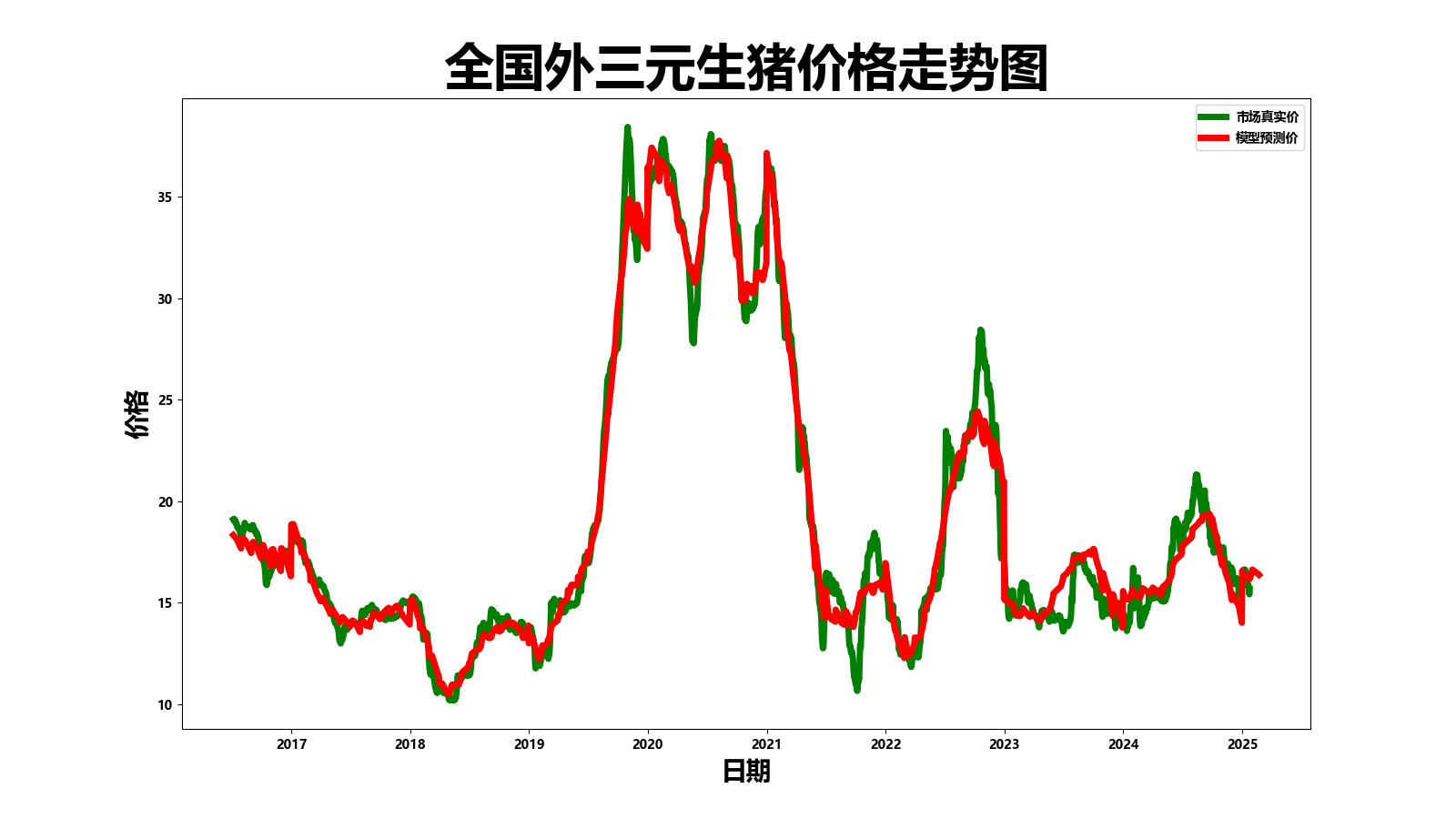
19  23/10/2016    17.12  16.24

Data Visualization

Python

import pandas as pd
import matplotlib
import matplotlib.pyplot as plt


matplotlib.use('TkAgg')
matplotlib.rc("font", family='MicroSoft YaHei', weight="bold")


def visualization():
    realDF = pd.read_table("../dataset/data", header=None, names=['dmy', 'price'], sep=" ")
    predictDF = pd.read_table("../dataset/predict", header=None, names=['dmy', 'price'], sep=" ")

    realDF['dmy'] = pd.to_datetime(realDF['dmy'], format="%d/%m/%Y")
    realDF.sort_values(by='dmy', inplace=True)

    predictDF['dmy'] = pd.to_datetime(predictDF['dmy'], format="%d/%m/%Y")
    predictDF.sort_values(by='dmy', inplace=True)

    plt.figure(figsize=(16, 9), dpi=100)
    plt.title("全国外三元生猪价格走势图", fontsize=40, weight="bold")
    plt.xlabel("日期", fontsize=20, weight="bold")
    plt.ylabel("价格", fontsize=20, weight="bold")
    plt.plot(realDF['dmy'], realDF['price'], '-g', linewidth=5.0, label="市场真实价")
    plt.plot(predictDF['dmy'], predictDF['price'], '-r', linewidth=5.0, label="模型预测价")
    plt.legend()
    plt.savefig("../model/output/trending_on_hog_price.png")
    plt.show()
    pass


if __name__ == '__main__':
    visualization()

Dataset & Full Code
Dataset and full code can be found on GitHub